IBonomics
Supply-Side Policy on AD–AS – Short-Run Demand Effect and Long-Run Growth
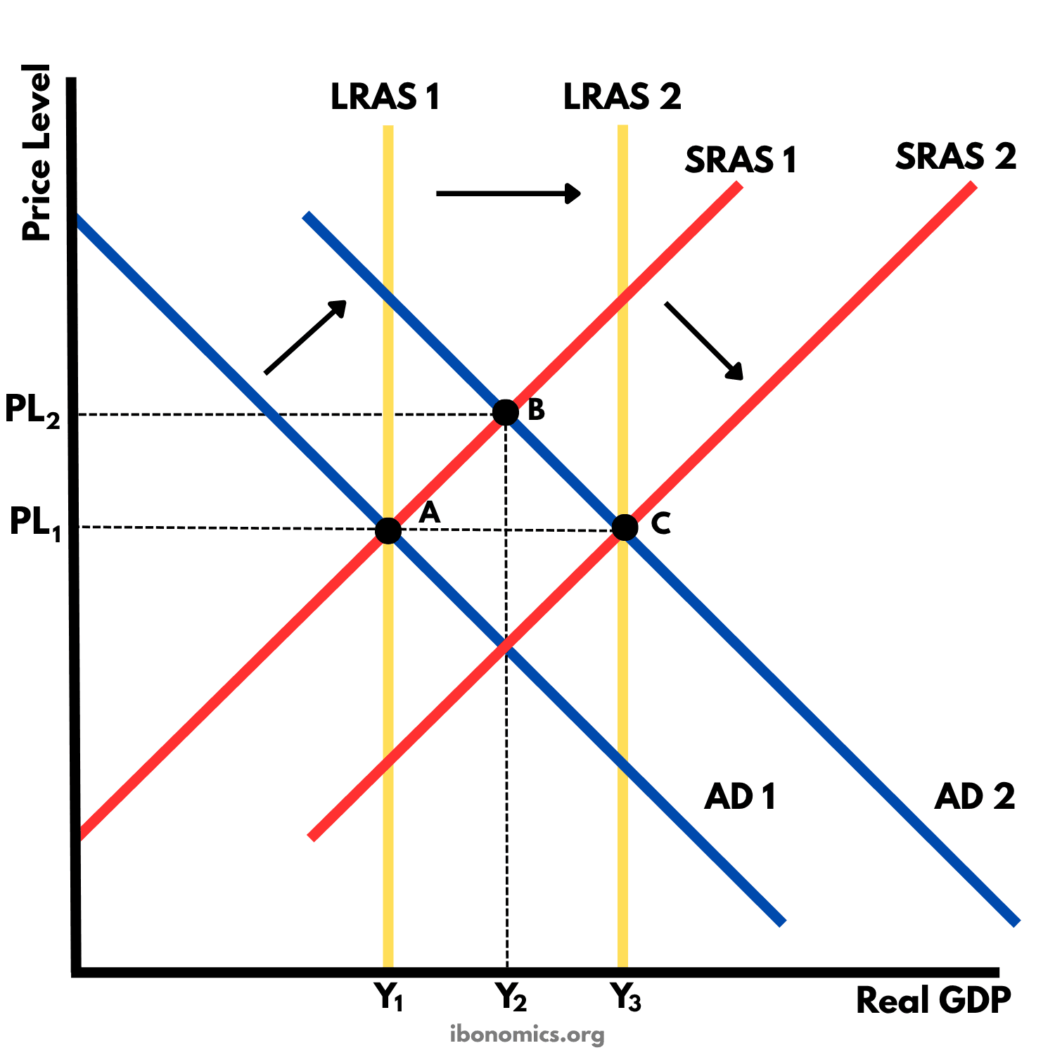
This diagram shows the short-run and long-run effects of an interventionist supply-side policy, such as government spending on infrastructure or education. In the short run, the spending raises aggregate demand, so real GDP and the price level rise from A to B. In the long run, the extra productive capacity shifts LRAS and SRAS right, so the economy reaches C, with real GDP higher at Y3.
Curves and elements
- AD 1
- Aggregate demand before the government spending.
- AD 2
- Aggregate demand after the spending, shifted right in the short run.
- LRAS 1
- Long-run aggregate supply, the economy's productive capacity before the policy.
- LRAS 2
- Long-run aggregate supply once the policy has increased productive capacity, shifted right.
- SRAS 1
- Short-run aggregate supply at the original level of costs.
- SRAS 2
- Short-run aggregate supply after the improvements lower firms' costs per unit, shifted right.
- PL1
- The price level at A and at C. The economy ends at PL1 here because capacity grows by as much as demand.
- PL2
- The short-run price level at B, where AD 2 meets SRAS 1.
- Y1
- Real GDP at A, the original full employment level.
- Y2
- Real GDP at B in the short run, beyond the original productive capacity.
- Y3
- Real GDP at C, the new full employment level.
- A
- The starting long-run equilibrium.
- B
- The short-run position after AD rises, before capacity has grown.
- C
- The new long-run equilibrium, where AD 2, SRAS 2 and LRAS 2 meet.
- Arrows
- The three shifts, all to the right. AD moves first, and LRAS and SRAS follow as capacity grows.
Key explanations
- 1
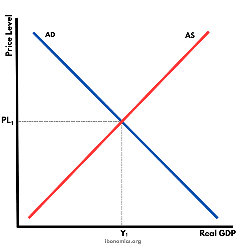
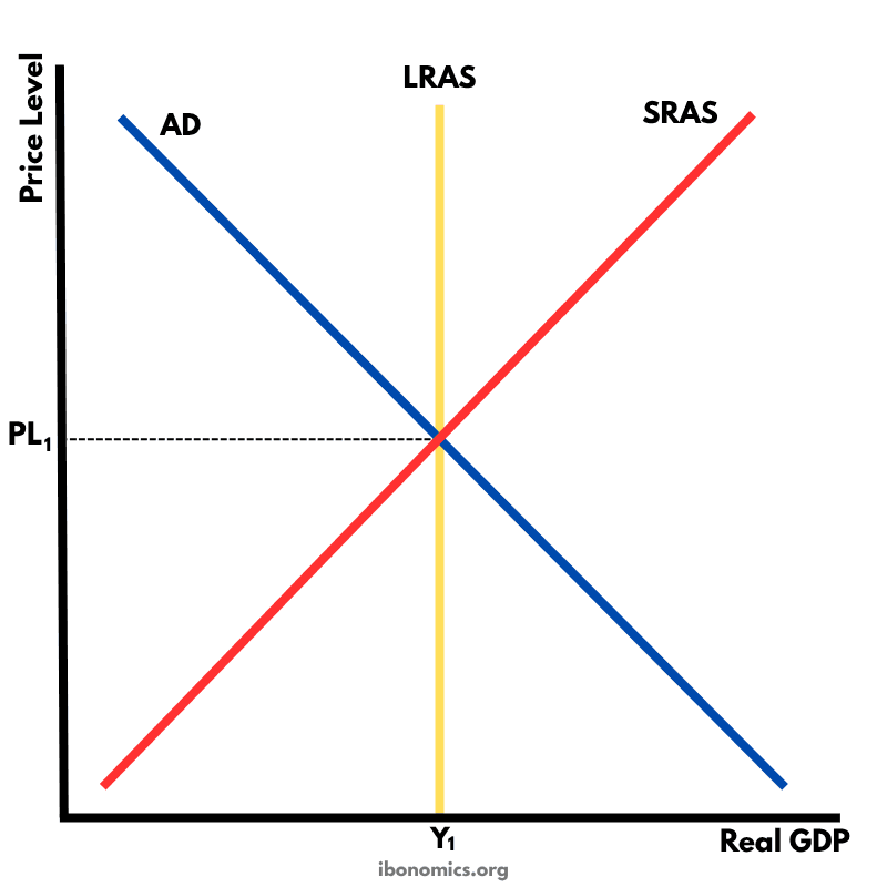
The economy starts in long-run equilibrium at A, where AD 1 meets SRAS 1 on LRAS 1, at real GDP Y1 and price level PL1.
- 2
The government spends on infrastructure or education. This spending is part of aggregate demand, so in the short run AD shifts right from AD 1 to AD 2. The economy moves from A to B, where real GDP rises to Y2, beyond the old productive capacity, and the price level rises to PL2.
- 3
Over time, the new roads, schools and skills increase the quantity and quality of the factors of production. The economy's productive capacity grows, so LRAS shifts right from LRAS 1 to LRAS 2.
- 4
The same improvements lower firms' costs per unit. Better infrastructure cuts transport costs, and a more skilled workforce produces more per hour, so SRAS also shifts right, from SRAS 1 to SRAS 2.
- 5
The economy reaches a new long-run equilibrium at C, where AD 2 meets SRAS 2 on LRAS 2. Real GDP is higher at Y3, so the growth lasts, unlike growth that comes from demand alone.
- 6
In this diagram the price level returns to PL1, because productive capacity grows by as much as demand. If capacity grows more than demand, the price level can end below PL1. If it grows less, the price level ends above PL1.
- 7
The main drawback is the time lag. The demand effect from A to B comes quickly, but the supply effect from B to C can take years, so in the meantime the policy adds to inflationary pressure. The spending also has an opportunity cost, and its success depends on choosing the right projects.
Example exam question
Using an AD/AS diagram, explain the short-run and long-run effects of government spending on infrastructure.
Show example answer
In the diagram, the economy starts at A, where AD 1 meets SRAS 1 on LRAS 1. Government spending on infrastructure is part of aggregate demand, so in the short run AD shifts right from AD 1 to AD 2, and the economy moves to B, with real GDP rising to Y2 and the price level to PL2. Over time, the new infrastructure increases the economy's productive capacity, shifting LRAS right from LRAS 1 to LRAS 2. It also lowers firms' costs, for example by cutting transport times, so SRAS shifts right from SRAS 1 to SRAS 2. The new long-run equilibrium is at C, with real GDP higher at Y3. Here the price level returns to PL1, because capacity grows by as much as demand, but it could end higher or lower depending on the relative size of the shifts. The main limitation is the time lag, because the supply-side benefits may take years to appear while the demand effect is immediate.